Active Inference, Entropy, Kalman filter, Expected free energy, Fundamental thermodynamic relation, Wondrous Wisdom
Andrius Kulikauskas investigates: What does free energy entail mathematically and metaphysically?
Starting with the math of free energy, I want to understand its conceptual significance, what is a natural interpretation of what it says. In this sense, I invert the "high road" and the "low road" of Active Inference, as I start at free energy rather than arrive at it. I have worked out the basic math. Currently, I am wondering where the probability distributions {$P(x,y)$} and {$Q(x)$} come from historically, as I don't find them in the physics literature. I am chasing them down through Karl Friston's work to Geoffrey Hinton's work and the origins of the Expectation Maximization algorithm.
Clarifying the Math of Active Inference and the Free Energy Principle
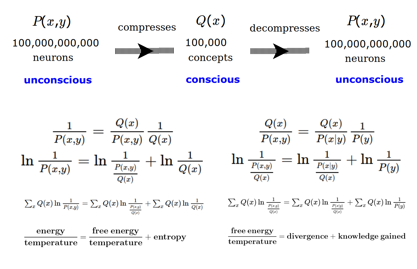
Free energy is defined in terms of two probability distributions, {$P(x,y)$} and {$Q(x)$}, where {$y$} is evidence and {$x$} is an inferred cause.
We can start with the formula that defines free energy.
| {$\frac{1}{P(x,y)} = \frac{Q(x)}{P(x,y)}\frac{1}{Q(x)}$} |
| {$\ln\frac{1}{P(x,y)} = \ln \frac{1}{\frac{P(x,y)}{Q(x)}} + \ln \frac{1}{Q(x)}$} |
| {$\ln \frac{1}{P(x,y)} = \ln \frac{Q(x)}{P(x,y)} + \ln \frac{1}{Q(x)}$} |
| {${\small \sum_x Q(x)\ln \frac{1}{P(x,y)} = \sum_x Q(x)\ln \frac{1}{\frac{P(x,y)}{Q(x)}} + \sum_x Q(x)\ln \frac{1}{Q(x)} }$} |
| {$\frac{\textrm{energy}}{\textrm{temperature}} = \frac{\textrm{free energy}}{\textrm{temperature}} + \textrm{entropy}$} |
We can think of these quantities as relating a knowledge lens and the knowledge gained.
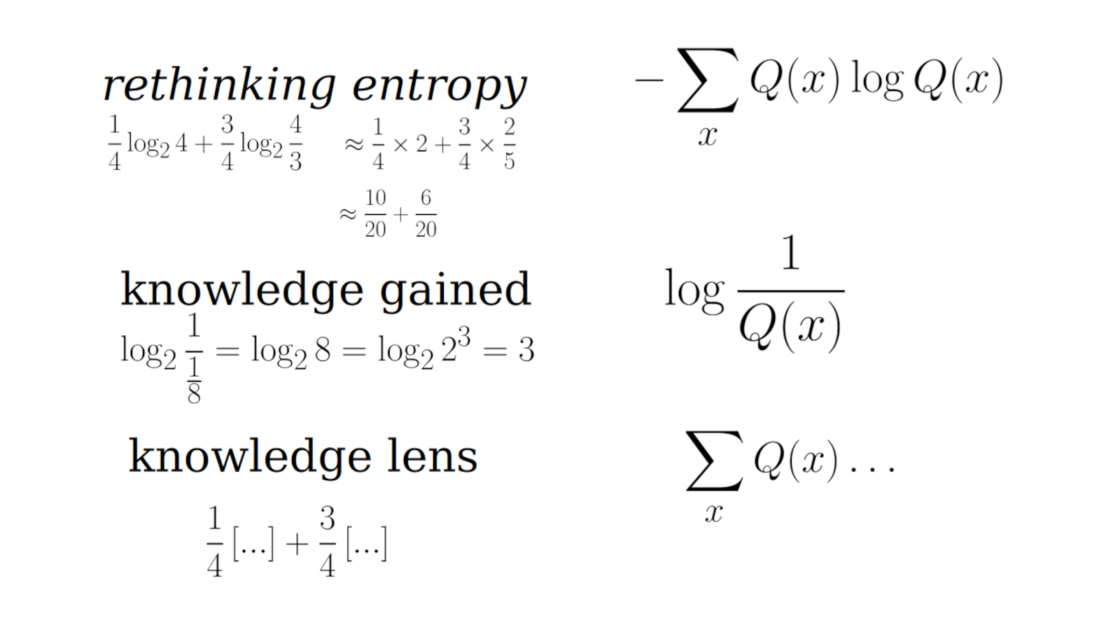
Entropy is a degenerate form of energy.
We can think of a dialogue between two levels of awareness, {$P(x,y)$} and {$Q(x)$}, where the latter compresses the former.
It makes sense that the knowledge lens be {$P(x,y)$} rather than {$Q(x)$}. I think this would be compatible with the theory of empowerment. But the math would be different so I would have to work that out.
The Active Inference framework variously breaks up free energy. The most usual is in terms of divergence and surprise. Thus free energy is an upper bound on surprise.
| {$P(x,y) = P(x|y)P(y)$} |
| {$\frac{Q(x)}{P(x,y)} = \frac{Q(x)}{P(x|y)}\frac{1}{P(y)}$} |
| {$\ln\frac{1}{\frac{P(x,y)}{Q(x)}} = \ln\frac{1}{\frac{P(x|y)}{Q(x)}} + \ln \frac{1}{P(y)}$} |
| {$\ln\frac{Q(x)}{P(x,y)} = \ln\frac{Q(x)}{P(x|y)} + \ln \frac{1}{P(y)}$} |
| {${\small \sum_x Q(x)\ln\frac{1}{\frac{P(x,y)}{Q(x)}} = \sum_x Q(x)\ln\frac{1}{\frac{P(x|y)}{Q(x)}} + \sum_x Q(x)\ln \frac{1}{P(y)} }$} |
| {$\frac{\textrm{free energy}}{\textrm{temperature}} = \textrm{divergence} + \textrm{knowledge gained}$} |
In the statistical jargon of the Wikipedia: Free energy principle this becomes:
| {$\sum_x Q(x)\ln\frac{Q(x)}{P(x,y)} = \sum_x Q(x)\ln\frac{Q(x)}{P(x|y)} + \ln \frac{1}{P(y)}\sum_x Q(x)$} |
| {$E_{Q(x)}\ln\frac{Q(x)}{P(x,y)} = E_{Q(x)}\ln\frac{Q(x)}{P(x|y)} + \ln \frac{1}{P(y)}$} |
| {$D_{KL}| Q(x) \parallel P(x,y)| = D_{KL}| Q(x) \parallel P(x|y) | + \ln \frac{1}{P(y)}$} |
| variational free energy {$=$} divergence {$+$} surprise |
Another way to break up free energy is in terms of accuracy and complexity.
Here we use {$P(x,y)=P(y|x)P(x)$} rather than {$P(x,y)=P(x|y)P(y)$}
{$F = \sum_x Q(x)\ln \frac{1}{\frac{P(x,y)}{Q(x)}} $}
{$F = \sum_x Q(x)\ln \frac{1}{\frac{P(y|x)P(x)}{Q(x)}}$}
{$F = \sum_x Q(x)\ln \frac{1}{P(y|x)} + \sum_x Q(x)\ln \frac{1}{\frac{P(x)}{Q(x)}}$}
Free energy = accuracy + complexity
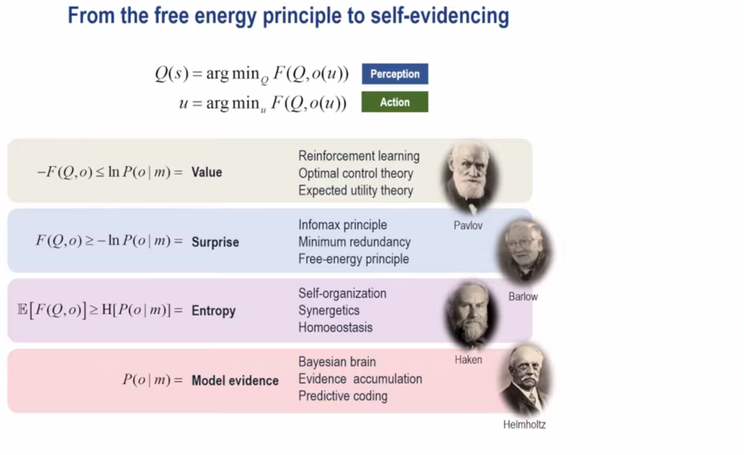
Friston writes this setting {$s=x$} and {$o=y$}. He notes this is an upper bound on surprise.
{$F = \sum_s Q(s)\ln \frac{1}{P(o|s)} + \sum_s Q(s)\ln \frac{Q(s)}{P(s)} \geq \ln \frac{1}{P(o)}$}
{$F = -\mathbb{E}_{Q(s)}[\ln P(o|s)] + D[Q(s)\parallel P(s)]\geq -\ln P(o)$}
{$-F = \mathbb{E}_{Q(s)}[\ln P(o|s)]-D[Q(s)\parallel P(s)]\leq \ln P(o)$}
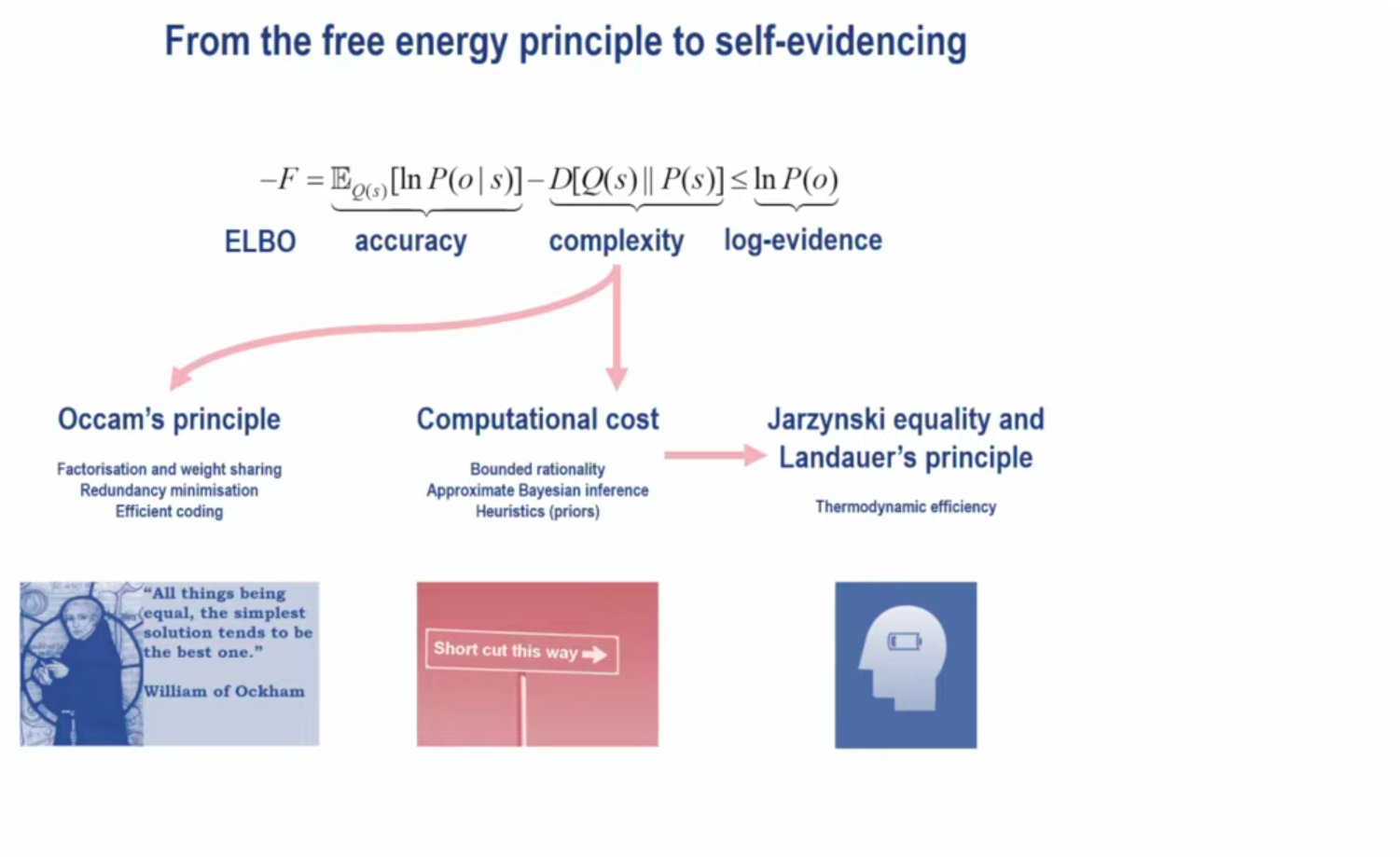
I don't understand how to derive this or what it actually says.
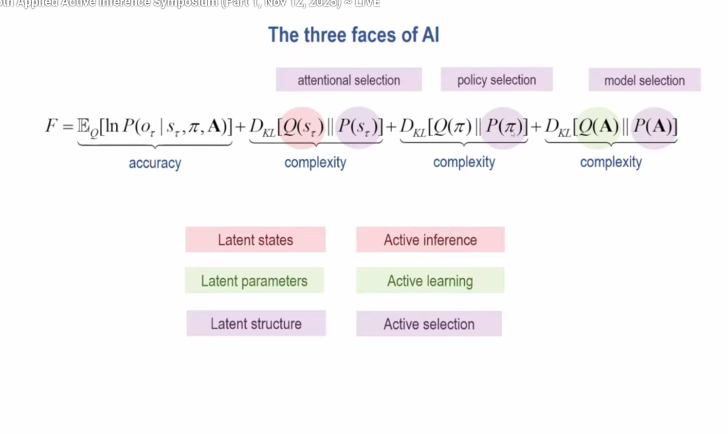
{$F=\mathbb{E}_Q[\ln P(o_\tau | s_\tau,\pi,A)] + D_{KL}[Q(s_\tau)\parallel P(s_\tau)] + D_{KL}[Q(\pi)\parallel P(\pi)] + D_{KL}[Q(A)\parallel P(A)]$}
{$F=\sum_\tau Q(s_\tau)\ln P(o_\tau | s_\tau,\pi,A) + \sum_\tau [Q(s_\tau)\ln\frac{Q(s_\tau)}{P(s_\tau)}] + \sum_\tau [Q(\pi)\ln\frac{Q(\pi)}{P(\pi)}] + \sum_\tau [Q(A)\ln\frac{Q(A)}{P(A)}]$}
In Active Inference, free energy is simply an upper bound on surprise.
Energy = free energy + entropy
Consequently:
Free energy = Energy - Entropy
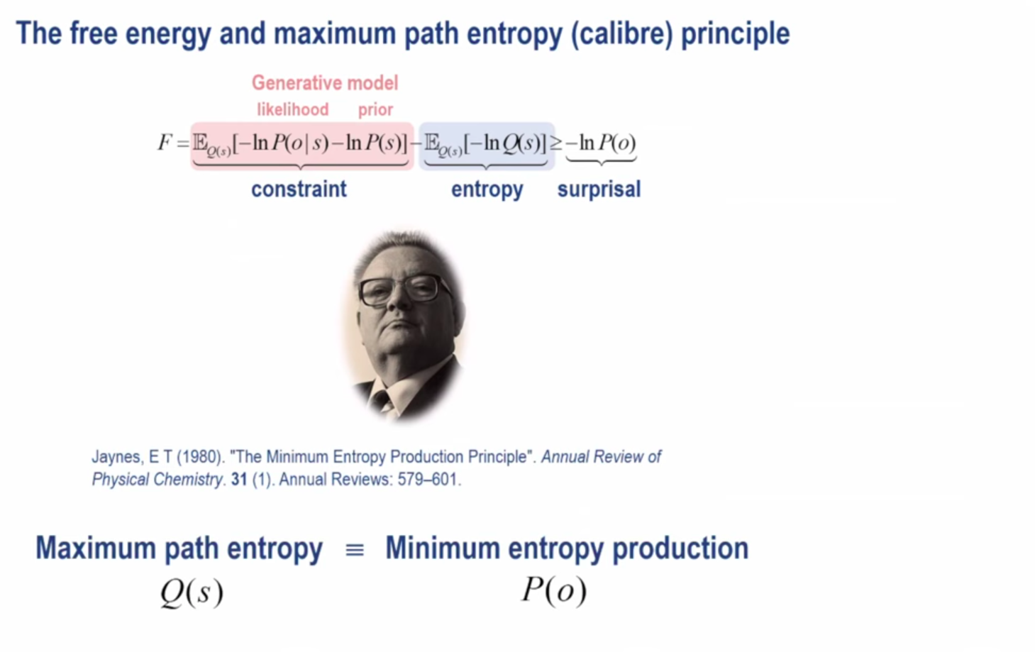
{$F = \sum_s Q(s)\ln \frac{1}{P(o,s)} - \sum_s Q(s)\ln \frac{1}{Q(s)}$}
{$F = \sum_s Q(s)\ln \frac{1}{P(o | s)P(s)} - \sum_s Q(s)\ln \frac{1}{Q(s)}$}
{$F = \sum_s Q(s)[\ln \frac{1}{P(o | s)} + \ln \frac{1}{P(s)}] - \sum_s Q(s)\ln \frac{1}{Q(s)}$}
{$F = \mathbb{E}_Q[-\ln P(o | s) - \ln P(s)] - \mathbb{E}_Q[-\ln Q(s)]\geq -\ln P(o)$}
He calls the energy "the constraint".
I don't understand the relation between {$Q(s)$} and {$P(o)$}.
He takes the expected value over {$t$}. I don't know if {$t$} is time. I don't understand how the surprisal becomes entropy.
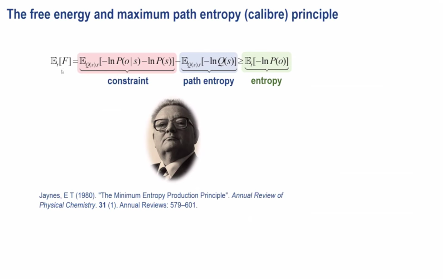
Free energy is {$F=\sum_\tau Q(s_\tau)\ln \frac{1}{\frac{P(s_\tau,o_\tau)}{Q(s_\tau)}}$}
{$P(s_\tau,o_\tau)= P(s_\tau)P(o_\tau | s_\tau)=P(o_\tau )P(s_\tau | o_\tau)$} can be understood in two ways.
{$F=\mathbb{E}_Q[\ln Q(s_\tau)-\ln P(s_\tau)-\ln P(o_\tau | s_\tau)]$}
{$F=\mathbb{E}_Q[\ln Q(s_\tau)-\ln P(s_\tau | o_\tau)-\ln P(o_\tau )]$}
Expected free energy
{$G=\mathbb{E}_Q[\ln Q(s_\tau | \pi)-\ln P(s_\tau)-\ln P(o_\tau | s_\tau)]$}
{$G(\pi)=\sum_\tau Q(s_\tau | \pi)\ln \frac{1}{\frac{P(s_\tau)}{Q(s_\tau | \pi)}} + \sum_\tau Q(s_\tau | \pi)\ln \frac{1}{P(o_\tau | s_\tau)}$}
{$G(\pi)=\sum_\tau Q(s_\tau | \pi)\ln \frac{1}{\frac{P(s_\tau,o_\tau)}{Q(s_\tau | \pi)}}$}
{$G=\mathbb{E}_Q[\ln Q(s_\tau | \pi)-\ln Q(s_\tau | o_\tau, \pi)-\ln P(o_\tau )]$}
{$G(\pi)=\sum_\tau Q(s_\tau | \pi)\ln \frac{1}{\frac{Q(s_\tau | o_\tau, \pi)}{Q(s_\tau | \pi)}} + \sum_\tau Q(s_\tau | \pi)\ln \frac{1}{P(o_\tau)}$}
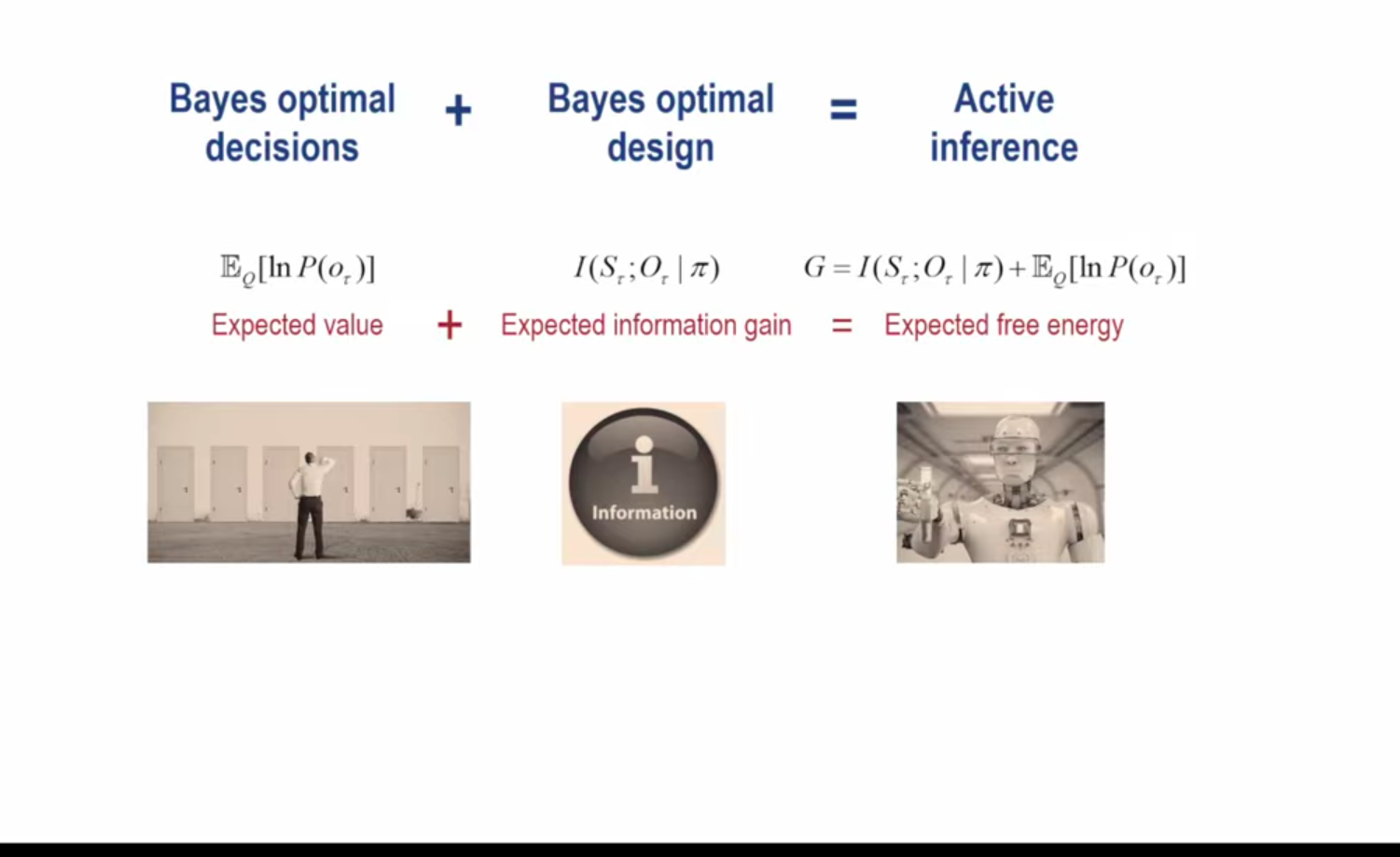
Expected free energy = expected information gain + expected value
{$G(\pi)=\sum_\tau Q(s_\tau | \pi)\ln \frac{1}{\frac{P(o_\tau)Q(s_\tau | o_\tau, \pi)}{Q(s_\tau | \pi)}}$}
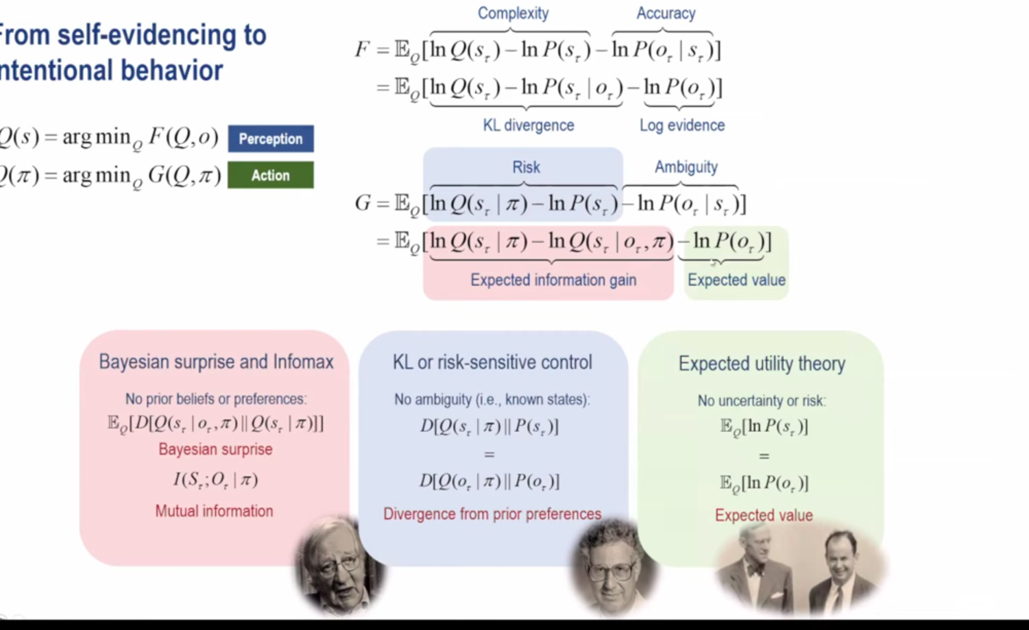
Expected information gain is defined above.
{$\mathbb{E}_Q[\ln P(\sigma_\tau)] + I(S_\tau;O_\tau | \pi) = G$}
{$\sum_\tau Q(o_\tau)\ln P(o_\tau) + I(S_\tau;O_\tau | \pi) = G$}
I don't understand what {$\mathcal{L}$} means.
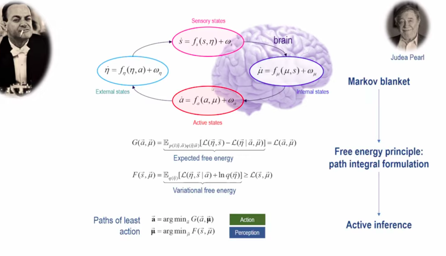
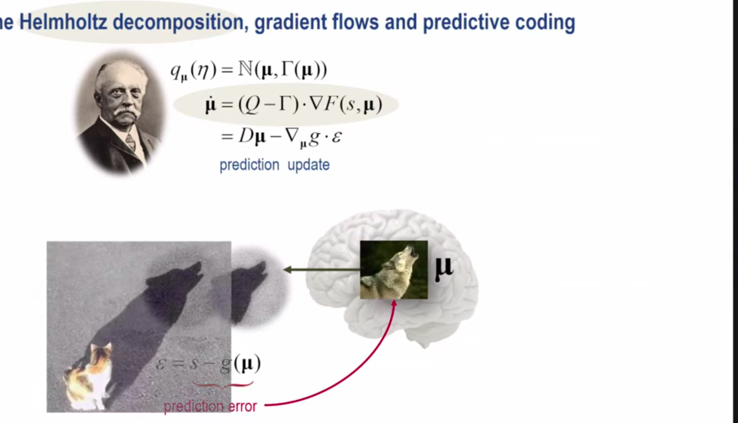
I need to study the Helmholtz decomposition.
The 2006 paper Karl Friston, James Kilner, Lee Harrison. A free energy principle for the brain., introduced the free energy principle. There the free energy has the form {$F=-\int q(\mathscr{v})\ln\frac{p(\tilde{y},\mathscr{v})}{q(\mathscr{v})}$}, with a continuous integral rather than a discrete sum. This paper cites the 2003 paper Karl Friston. Learning and inference in the brain. which has the same formula and cites the 1976 paper A.P.Dempster, N.M.Laird, D.B.Rubin. Maximum Likelihood from Incomplete Data via the EM Algorithm. This latter paper calculates maximum likelihoods with a two-step algorithm, consisting of an expectation-step and a maximization-step. Equation 2.6 is perhaps a key equation for maximizing {$L(\phi)=\log f(x|\phi)-\log \frac{f(x|\phi)}{g(y|\phi)}$}, which is perhaps minimizing free energy {$-L(\phi)=\log \frac{g(y|\phi)}{f(x|\phi)} + \log \frac{1}{f(x|\phi)}$} as divergence plus knowledge gained. The 2003 paper also cites the work of Geoffrey Hinton. A paper not cited but yet helpful and relevant is Geoffrey E. Hinton, Richard S. Zemel. Autoencoders, Minimum Description Length and Helmholtz Free Energy.
It seems that the EM algorithm showed the significance of the combination of divergence and knowledge gained. Hinton recognized that the quantity which is minimized is the free energy. Friston then developed the Free Energy Principle as a general principle which organisms apply to make the most of that combination. But I would want to consider what this truly means in terms of energy and entropy, the formula that I considered.
Earlier notes
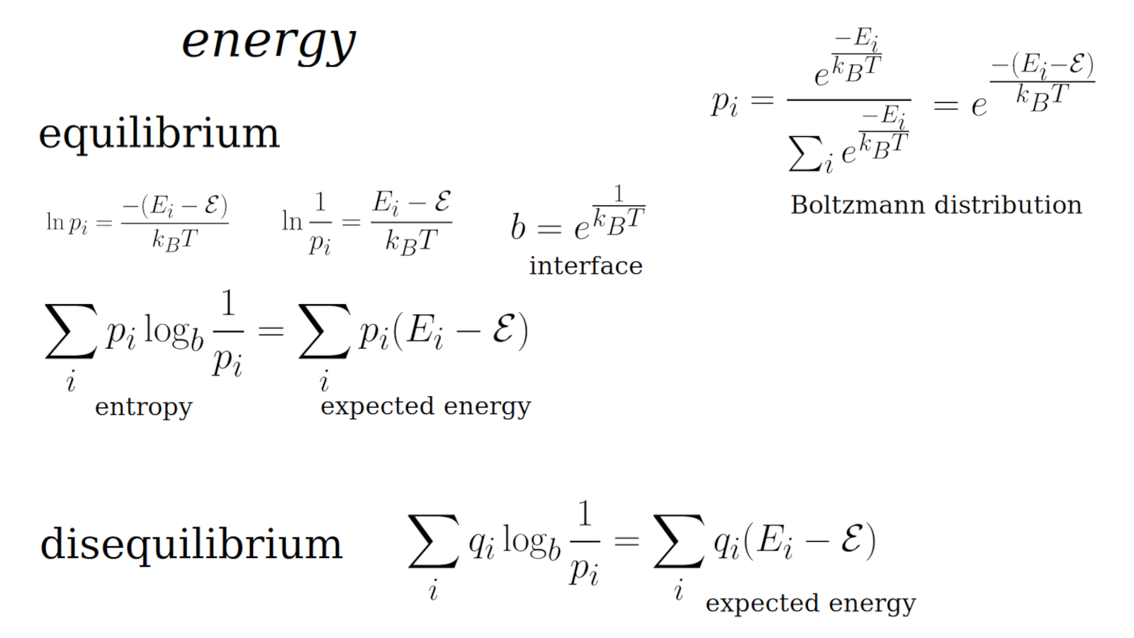
{$p_i = e^{-H_i}$}
{$\frac{1}{p_i}=e^{H_i}$}
{$\ln \frac{1}{p_i}=H_i$}
with temperature, which gives the base for the log
{$p_i = e^{-\frac{H_i}{T}}$}
{$\frac{1}{p_i}=e^{\frac{1}{T}}e^{H_i} = (e^{\frac{1}{T}})^{H_i} $}
{$\ln \frac{1}{p_i}=\frac{1}{T}H_i$}
Actually, we must divide by the normalization, the canonical partition function {$Z=\sum_x e^{-\frac{p_x}{T}}$} where I have set Boltzmann's constant to {$1$}.
{$p_i = \frac{1}{Z}e^{-\frac{H_i}{T}}$}
We can compare two different probabilities and then we don't have to worry about {$Z$}.
Energy is the knowledge gained. It expresses the probability of being found in the state. The smaller the probability, the larger the energy. This makes sense especially if we suppose it started in that state, in which case it would be the perturbability, thus the graduated improbability. But we don't assume it started in that state but so it is simply the probability of getting in that state.
{$\sum_x Q(x)H(x)$} is the expected energy, which is the cross entropy.
- John C. Baez, Blake S. Pollard. Relative Entropy in Biological Systems.
- John Baez. Relative entropy (structures), functor on statistical inference, functor, wrap-up
- John Baez video mentioning relative entropy
- John Baez, Tobias Fritz. A Bayesian Characterization of Relative Entropy.
- Tom Leinster. A short characterization of relative entropy.
Relative entropy is the Kullback-Leibler divergence. {$\sum_x Q(x) \log\frac{1}{\frac{P(x)}{Q(x)}}$}
It is the expected amount of information that you gain when you thought the right probability distribution was P(x) and you discover it is really Q(x).
Tom Leinster. An Operadic Introduction to Entropy.
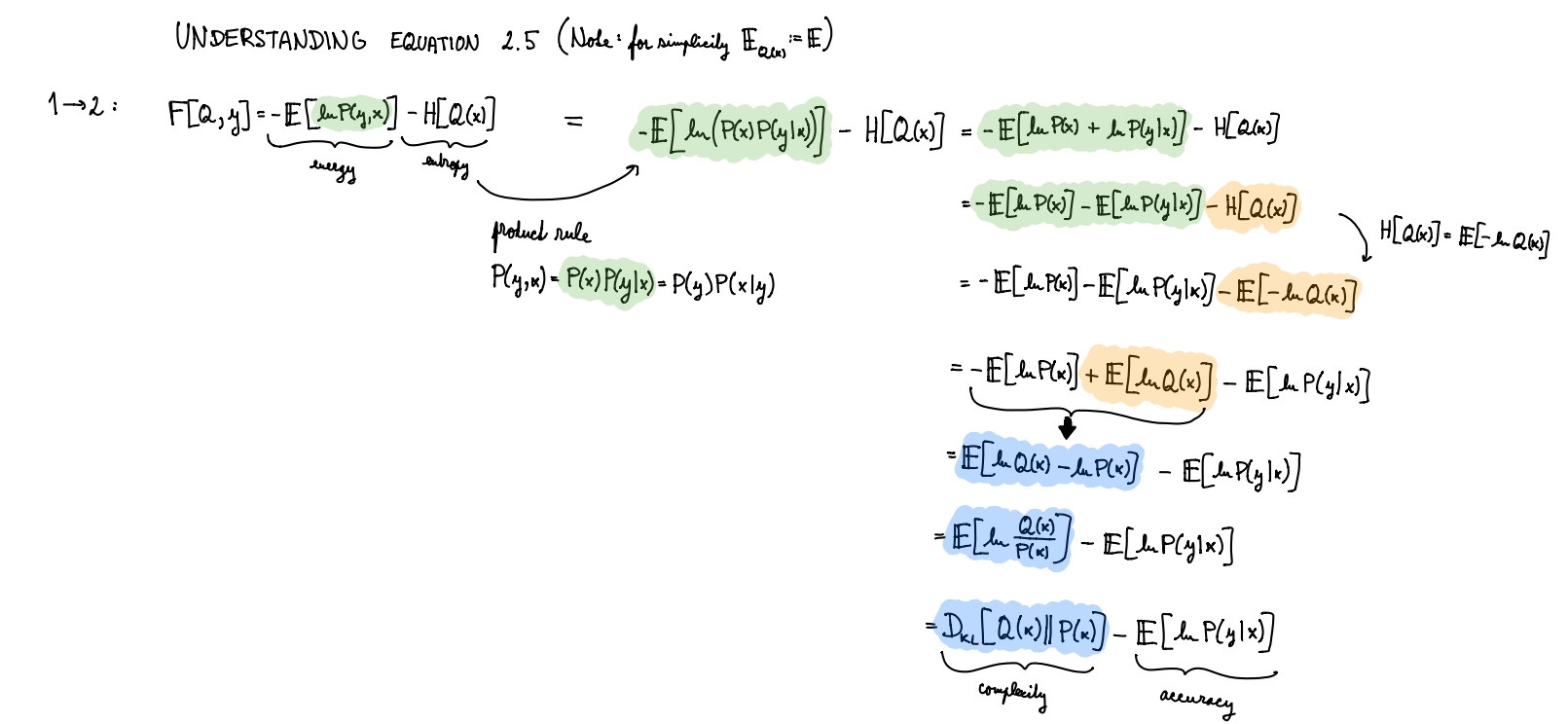
| {$=\sum_x [Q(x)\ln\frac{1}{P(x,y)} - Q(x)\ln\frac{1}{Q(x)}]$} | variational free energy | |
| {$=\sum_x [Q(x)\ln\frac{1}{P(x)P(y|x)} - Q(x)\ln\frac{1}{Q(x)}]$} | focus on cause and then evidence | |
| {$=\sum_x [Q(x)(\ln\frac{1}{P(x)} - \ln\frac{1}{Q(x)}) + Q(x)\ln\frac{1}{P(y|x)}]$} | ||
| {$=\sum_x [Q(x)(\ln Q(x) - \ln P(x)) - Q(x)\ln P(y|x)]$} | complexity minus accuracy |
| {$=\sum_x [Q(x)(\ln Q(x) - \ln P(x)) - Q(x)\ln P(y|x)] + \ln P(y)$} | add a constant {$\ln P(y)$} | |
| {$=\sum_x [Q(x)(\ln Q(x) - \ln P(x)) - Q(x)\ln P(y|x)] + \ln P(y)\sum_x Q(x)$} | multiply by {$1 = \sum_x Q(x)$} | |
| {$=\sum_x [Q(x)(\ln Q(x) - \ln P(x)) - Q(x)\ln P(y|x)] + Q(x)P(y)$} | reorganize | |
| {$=\sum_x [Q(x)(\ln Q(x) - \ln P(x)) + Q(x)(\ln P(y) - \ln P(y|x)]$} | conceptual inadequacy plus prediction error |
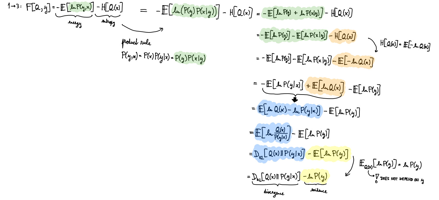
| {$=\sum_x [Q(x)\ln\frac{1}{P(x,y)} - Q(x)\ln\frac{1}{Q(x)}]$} | variational free energy | |
| {$=\sum_x [Q(x)\ln\frac{1}{P(y)P(x|y)} - Q(x)\ln\frac{1}{Q(x)}]$} | focus on evidence and then cause | |
| {$=\sum_x [Q(x)(\ln\frac{1}{P(x|y)} - \ln\frac{1}{Q(x)}) + Q(x)\ln\frac{1}{P(y)}]$} | divergence plus surprise | |
| {$=\sum_x [Q(x)(\ln Q(x) - \ln P(x|y)) - Q(x)\ln P(y)]$} | divergence minus evidence |
other notes...
| {$=\sum_x [Q(x|y)\textrm{ln}\frac{1}{P(x|y)} - Q(x|y)\textrm{ln}\frac{1}{Q(x|y)}]$} | definition of free energy as energy minus entropy | |
| {$=\mathbb{E}_{Q(x|y)}[\textrm{ln}Q(x|y)-\textrm{ln}P(x|y)]$} | logarithm product rule, definition of expected value | Helmholtz free energy: entropy minus energy |
| {$=\mathbb{E}_{Q(x|y)}[\textrm{ln}Q(x|y)-\textrm{ln}P(y|x)-\textrm{ln}P(x)+\textrm{ln}P(y)]$} | Bayes's rule | |
| {$=\mathbb{E}_{Q(x|y)}[\textrm{ln}Q(x|y)-\textrm{ln}P(x)]+\mathbb{E}_{Q(x|y)}[\textrm{ln}P(y)-\textrm{ln}P(y|x)]$} | reorganize | deviation plus prediction error |
| {$=\mathbb{E}_{Q(x|y)}[\textrm{ln}Q(x|y)-\textrm{ln}P(x)]+\mathbb{E}_{Q(x|y)}[-\textrm{ln}P(y|x)]+\textrm{ln}P(y)$} | realize {$\textrm{ln}P(y)$} is independent of {$Q(x|y)$} | |
| {$=D_{KL}[Q(x|y)\parallel P(x)]+\mathbb{E}_{Q(x|y)}[-\textrm{ln}P(y|x)]+\textrm{ln}P(y)$} | definition of KL divergence, independence of {$P(y)$} from {$x$} |
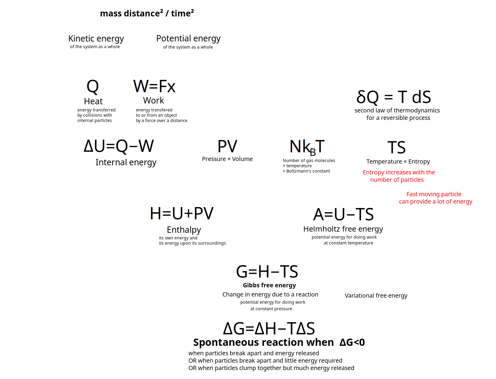
In physics
| {$A=U-TS$} | Helmholtz free energy {$A$}, internal energy {$U$}, temperature {$T$}, entropy {$S$} | |
| {$\frac{A}{T}=\frac{U}{T}-S$} | divide by temperature, focus on entropy | |
| {$=\sum_x [Q(x)\textrm{ln}\frac{1}{P(x,y)} - Q(x)\textrm{ln}\frac{1}{Q(x)}]$} | variational free energy |
- Free energy is the portion of any first-law energy that is available to perform thermodynamic work at constant temperature, i.e., work mediated by thermal energy.
- The change in the free energy is the maximum amount of work that the system can perform in a process at constant temperature.
- Its sign indicates whether the process is thermodynamically favorable or forbidden.
- Helmholtz free energy {$A=U-TS$}
- {$U$} is the internal energy of a thermodynamic system. It excludes the kinetic energy of motion of the system as a whole and the potential energy of position of the system as a whole. It includes the thermal energy, i.e., the constituent particles' kinetic energies of motion ( translations, rotations, and vibrations) relative to the motion of the system as a whole. It also includes potential energies associated with microscopic forces, including chemical bonds.
- In general, {$U$} is the energy of a system as whole and not as the subsystem within a greater whole.
- Entropy is defined as {$S=-k_B\sum_ip_i\ln p_i$} where {$k_B=1.380649×10^{−23}$} joules per kelvin and {$p_i$} is the probability that state {$i$} of a system is occupied. We can eliminate the minus sign by writing {$\textrm{ln}\frac{1}{p_i}$}.
- Free energy is related to potential energy whereas entropy is related to kinetic energy.
- Under a Boltzmann distribution, the average log probability of a system adopting some configuration is inversely proportional to the energy associated with that configuration—that is, the energy required to move the system into this configuration from a baseline configuration
Consider the correspondence of a world of evidence (known through our senses) and a world of causes (not known but inferred).
- {$y$} is the evidence What, what is known, what the answering mind observers, the observation, for example, "jumping" or "not moving".
- {$x$} is the cause How, what is not known, what the questioning mind supposes, what is the subject of belief or hypothesis, for example, "a frog" or "an apple".
- {$x$} is an estimate of features, of an agent
We start with the prior belief {$P(x)$} regarding cause {$x$}. Given new evidence {$y$}, we want to calculate the new belief, the posterior belief {$P(x|y)$} regarding cause {$x$}.
We conflate the two worlds by considering them both in terms of probabilities.
- {$P(x)$} is the probability of the cause. It is the prior belief. (Regarding How)
- {$P(x|y)$} is the probablity of the cause given the evidence. It is the posterior belief. (Regarding Why)
- {$P(y)$} is the probability of the evidence. It is called the marginal probability or the model evidence. (Regarding What)
- {$P(y|x)$} is the probability of the evidence given the cause. It is called the likelihood. (Regarding Whether)
- {$P(x,y)$} is the probability of the evidence and the cause.
Bayes's theorem states
- {$P(x,y)=P(x)P(y|x)=P(y)P(x|y)$}
Marginalization states that summing over all possible {$x$} gives:
- {$\sum_x P(x,y)=\sum_x P(y)P(x|y)=P(y)\sum_x P(x|y)=P(y)$}
This means that we can calculate the model evidence (the probability of the evidence) by summing the combined probability (for evidence {$y$} and cause {$x$}) over all of the causes {$x$}. But also:
- {$P(y)=\sum_x P(x,y)=\sum_x P(x)P(y|x)$}
This means that we can calculate the model evidence (the probability of the evidence) by summing over all causes {$x$} the product of the prior belief and the likelihood.
The generative model consists of the prior belief {$P(x)$} and the likelihood {$P(y|x)$}.
- They yield a sensory output of what we predict to see in the world, which we can compare with what we then actually do see.
- From them by marginalization we can calculate the model evidence {$P(y)$}.
- And then using Bayes's theorem we can calculate the posterior belief {$P(x|y)$}. That is the goal!
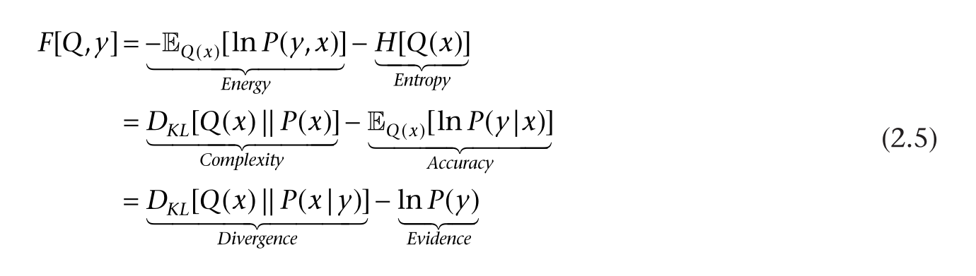
Variational free energy {$F[Q,y]$}
- It is a function of the questioning mind's approximation of the posterior belief {$Q$} and the answering mind's evidence {$y$}.
- It is the sum of the prediction error {$u'-u$} (how much the generative model's outputted prediction {$u'$} differs from the latest sensory data {$u$}) and the deviation {$D_{KL}(v'|v_{prior})$} of the posterior inferred cause {$v'$} from the prior inferred cause {$v$}.
- {$=\mathbb{E}_Q[\textrm{ln}Q(x|y)-\textrm{ln}P(x)]+\mathbb{E}_Q[-\textrm{ln}P(y|x)]+\textrm{ln}P(y)$}
- The predicted error is given by {$\mathbb{E}_Q[-\textrm{ln}P(y|x)]+\textrm{ln}P(y)$}. This subtracts from the observation {$y$} the particular cause {$x$}, thus sums over all other causes.
- The deviation compares, for each cause {$x$}, the approximate posterior belief in that cause {$\textrm{ln}Q(x|y)$}, supposing observation {$y$}, with the prior belief in that cause {$\textrm{ln}P(x)$}.
- Divergence minus evidence: {$D_{KL}[Q(x)\parallel P(x|y)] - \textrm{ln}P(y)$}. Free energy is minimized when divergence decreases and evidence increases (approaches 1).
- Divergence plus prediction error.
- Alternatively, is the complexity minus accuracy: {$D_{KL}[Q(x)\parallel P(x)] - \mathbb{E}_{Q(x)}[\textrm{ln}P(y|x)]$} complexity is the degree the approximation for the posterior belief does not match up with the prior belief, and accuracy is the extent the likelihood overlaps with the approximation for the posterior belief. Free energy is minimized when complexity decreases and accuracy increases.
- From the physical point of view, is energy minus entropy:
- {$\sum_xQ(x|y)\textrm{ln}[Q(x|y)] - \sum_xQ(x|y)\textrm{ln}P(x|y)$} which is entropy minus energy
- {$-\mathbb{E}_{Q(x)}[\textrm{ln}P(y,x)]-H[Q(x)]$}.
- Comparing with the other definitions, this can be written as minus entropy (which expresses the questioning mind and the approximation) plus energy (which expresses the answering mind and the evidence). Free energy is minimized when energy decreases and entropy increases. According to the second law of thermodynamics, entropy stays the same or increases.
- This is Helmholtz free energy {$U-TS$}, where {$U$} is the internal energy of the system, {$T$} is the temperature, and {$S$} is the entropy. This measures the useful work obtainable from a closed thermodynamic system at a constant temperature. It thus allows for pressure changes, as with explosives. Whereas Gibbs free energy, relevant for chemical reactions, assumes constant pressure, allowing for temperature changes.
Minimize free energy by adjusting the paramaters {$\phi$}.
{$P$} describes the probabilities given by the first mind, the neural mind, which knows the actuality
{$Q$} approximates {$P$} to calculate the posterior belief
- {$Q$} describes the probabilities given by the second mind, the conceptual mind, which is modeling the actuality. We have {$P\sim Q$}.
- {$Q$} is a guess, an inference, that approximates the posterior belief {$Q(v|u)\sim P(v|u)$}.
- Use approximate posterior {$q$} and learn its parameters (synaptic weights) {$\phi $}.
My ideas
- Think of {$Q(x)$} as modeling the state of full knowledge of observations. Thus {$Q(y)=1$} and {$Q(x|y)=Q(x)$}. Thus we are comparing {$P(x|y)$} with {$Q(x)$}.
- In this spirit, we can write:
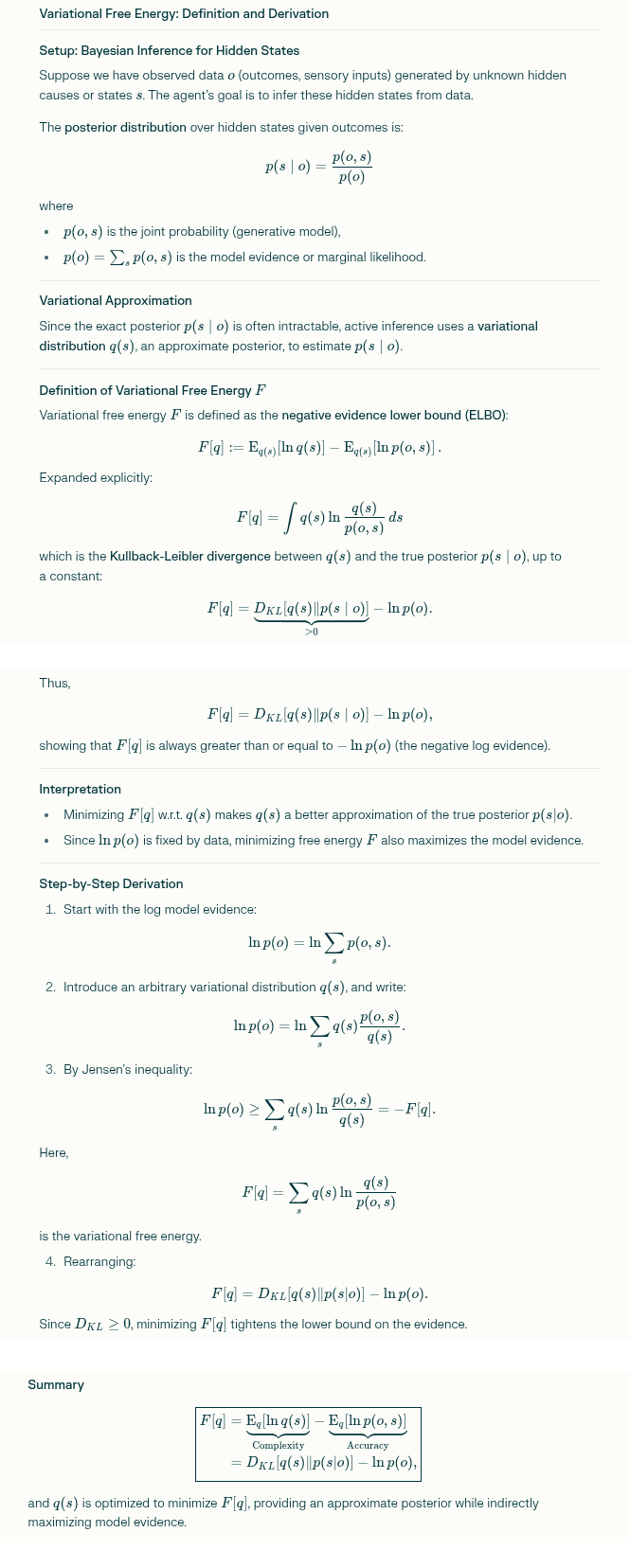
{$\textrm{ln}P(y)=\textrm{ln}\sum_x P(y,x)\frac{Q(x)}{Q(x)}=\textrm{ln}\mathbb{E}_{Q(x)}\left [\frac{P(y,x)}{Q(x)}\right ]$} and by Jensen's inequality
{$\geq \mathbb{E}_{Q(x)}\left [\textrm{ln}\frac{P(y,x)}{Q(x)}\right ] = -F[Q,y]$} which is the negative of the free energy
Recalling that {$P(x,y)=P(y)P(x|y)$} we have:
{$\textrm{ln}P(x,y)=\textrm{ln}P(y) + \textrm{ln}P(x|y)$} implies
{$\mathbb{E}_{P(x|y)}[\textrm{ln}P(x,y)]=\textrm{ln}P(y)+\mathbb{E}_{P(x|y)}[\textrm{ln}P(x|y)]$}
and comparing {$Q(x)$} with {$P(x|y)$} and recalling the definition of {$F[Q,y]=\mathbb{E}_{Q(x|y)}[\textrm{ln}\frac{Q(x,y)}{P(x,y}$} we can compare
{$\mathbb{E}_{Q(x)}[\textrm{ln}P(x,y)]= -F[Q,y] + \mathbb{E}_{Q(x)}[\textrm{ln}Q(x)]$}
From this perspective, the free energy {$F[Q,y]$} expresses {$\textrm{ln}\frac{P(x|y)}{P(x,y)}=\textrm{ln}\frac{1}{P(y)}=-\textrm{ln}P(y)$}. The probability {$P(y)\leq 1$} and so {$-\textrm{ln}P(y)\geq 0$}. Minimizing the free energy means increasing the certainty {$P(y)$}. Zero free energy means that {$P(y)=1$} is certain. And this is the aspiration for {$Q(x)$}, that it includes the observation {$y$}.
KL Divergence
- Proof that KL-divergence is non-negative
- KL Divergence is also known as (Shannon) Relative Entropy.
- KL Divergence characterizes information gain when comparing statistical models of inference.
- KL Divergence expresses the expected excess surprisal from using {$Q$} as a model instead of {$P$} when the actual distribution is {$P$}.
- KL Divergence is the excess entropy. It is the expected extra message-length per datum that must be communicated if a code that is optimal for a given (wrong) distribution {$Q$} is used, compared to using a code based on the true distribution {$P$}.
- KL Divergence is a measure of how much a model probability distribution {$Q$} is different from a true probability distribution {$P$}.
- {$$D_{KL}(P\parallel Q)=\sum_{x\in X}P(x)\textrm{log}\frac{P(x)}{Q(x)}$$}
- Minimize the Kullback-Leibler divergence ('distance') between {$Q$} and true Posterior {$P$} by changing the parameters {$\phi$}.
Notation: {$u=y$} is the evidence and {$v=x$} is the cause. Bayes theorem lets us calculate the posterior belief: {$P(v|u)=\frac{P(u|v)P(v)}{P(u)}$}
Given an observation {$x$} and a cause {$y$}, we want to minimize the divergence of the conceptual model {$Q(x|y)$} from the sensory data {$P(x|y)$}.
(Appendix B.2)
- States {$s$} influence outcomes (evidence) {$o$}
- Free energy is a functional of two things: approximate posterior beliefs ({$Q$}) and a generative model ({$P$}).
- Free energy for a given policy {$\pi$} is: {$F(\pi)=E_{Q(\tilde{s}|\pi)}[\ln Q(\tilde{s}|\pi)-\ln P(\tilde{o},\tilde{s}|\pi)]$}
- {$F(\pi)\geq -\ln P(\tilde{o}|\pi)$}
- {$Q(\tilde{s}|\pi)=\underset{Q}{\textrm{arg}\;\textrm{min}\;} F(\pi)\Rightarrow F(\pi)=-\ln P(\tilde{o}|\pi)$}
Mathematical definition of free energy
| {$D_{KL}[Q(x|y)\parallel P(x|y)]$} | definition of free energy | |
| {$=\sum_x Q(x|y)\textrm{ln} \left [\frac{Q(x|y)}{P(x|y)} \right ]$} | definition of KL divergence | |
| {$=\mathbb{E}_{Q(x|y)}[\textrm{ln}Q(x|y)-\textrm{ln}P(x|y)]$} | logarithm product rule, definition of expected value | Helmholtz free energy: entropy minus energy |
| {$=\mathbb{E}_{Q(x|y)}[\textrm{ln}Q(x|y)-\textrm{ln}P(y|x)-\textrm{ln}P(x)+\textrm{ln}P(y)]$} | Bayes's rule | |
| {$=\mathbb{E}_{Q(x|y)}[\textrm{ln}Q(x|y)-\textrm{ln}P(x)]+\mathbb{E}_{Q(x|y)}[\textrm{ln}P(y)-\textrm{ln}P(y|x)]$} | reorganize | deviation plus prediction error |
| {$=\mathbb{E}_{Q(x|y)}[\textrm{ln}Q(x|y)-\textrm{ln}P(x)]+\mathbb{E}_{Q(x|y)}[-\textrm{ln}P(y|x)]+\textrm{ln}P(y)$} | realize {$\textrm{ln}P(y)$} is independent of {$Q(x|y)$} | |
| {$=D_{KL}[Q(x|y)\parallel P(x)]+\mathbb{E}_{Q(x|y)}[-\textrm{ln}P(y|x)]+\textrm{ln}P(y)$} | definition of KL divergence, independence of {$P(y)$} from {$x$} |
Note that {$\textrm{ln}P(y)$} is constant with respect to {$x$}.
The free energy is {$D_{KL}[Q(x|y)\parallel P(x)]+\mathbb{E}_Q[-\textrm{ln}P(y|x)]$}. It combines the conceptual discrepancy and the sensory discrepancy.
Conceptual discrepancy
- {$D_{KL}[Q(v|u)\parallel P(v)]$} {$KL$}-divergence of prior and posterior ... the internal discrepancy in the questioning mind
Sensory discrepancy
- {$\mathbb{E}_Q[-\textrm{ln}P(u|v)]$} how surprising is the sensory data ... the external discrepancy in the answering mind
{$p_\nu = \frac{e^{-\beta E_\nu}}{Z}$} probability of being in the energy state {$E_\nu$} (Boltzmann distribution)
{$-\textrm{ln}P(x,y)$} energy of the explanation
{$\sum_x Q(x|y)[-\textrm{ln}P(x,y)]$} average energy
{$\sum_x -Q(x|y)\textrm{ln}Q(x|y)$} entropy
Active Inference Textbook Equation 2.5
I got the answer below from Perplexity AI.
Free energy
Andrius: I am studying the different kinds of energy so that I could understand free energy, which is basic for Active Inference.
Internal energy {$U$} has to do with energy on the microscopic scale, the kinetic energy and potential energy of particles.
Heat {$Q$} has to do with energy transfer on a macroscopic scale across a boundary.
See also: Active Inference at Math 4 Wisdom
People to work with
Active Inference Math Learning Group
Jonathan Shock, Associate Professor, Mathematics and Applied Mathematics, University of Cape Town
Active Inference Textbook Math Equations with explanations
Did Jakub Smékal do the math equation derivations?
- Karl Friston, Jérémie Mattout, Nelson Trujillo-Barreto, John Ashburner, Will Pennya. Variational free energy and the Laplace approximation.
- Statistical Parametric Mapping software documentation
- A Worked Example of the Bayesian Mechanics of Classical Objects
- Some interesting observations on the free energy principle
- Karl Friston. Active inference and belief propagation in the brain. Equations
Literature
- Sebastian Gottwald, Daniel A. Braun. The two kinds of free energy and the Bayesian revolution.
- Luca M. Possati. Markov Blanket Density and Free Energy Minimization
- Karl Friston, Lancelot Da Costa, Noor Sajid, Conor Heins, Kai Ueltzhöffer, Grigorios A. Pavliotis, Thomas Parr. The free energy principle made simpler but not too simple.
- Thomas Parr, Giovanni Pezzulo, Rosalyn Moran, Maxwell Ramstead, Axel Constant, Anjali Bhat. Five Fristonian Formulae.
- Ariel Cheng. Explaining the Free Energy Principle to my past self. Part I: Things
- Karl Friston, Lancelot Da Costa, Dalton A.R. Sakthivadivel, Conor Heins, Grigorios A. Pavliotis, Maxwell Ramstead, Thomas Parr. Path integrals, particular kinds, and strange things.
- Matthew J. Beal. Variational Algorithms for Approximate Bayesian Inference.
- Andrew Gelman, John B. Carlin, Hal S. Stern, David B. Dunson, Aki Vehtari, Donald B. Rubin. Bayesian Data Analysis. Third edition.
- Takuya Isomura, Karl Friston. Reverse-Engineering Neural Networks to Characterize Their Cost Functions.
- Karl J. Friston, Tommaso Salvatori, Takuya Isomura, Alexander Tschantz, Alex Kiefer, Tim Verbelen, Magnus Koudahl, Aswin Paul, Thomas Parr, Adeel Razi, Brett Kagan, Christopher L. Buckley, Maxwell J. D. Ramstead. Active Inference and Intentional Behaviour.
Critique
History
- Geoffrey Hinton, Richard Zemel. Autoencoders, Minimum Description Length and Helmholtz Free Energy.
- Peter Dayan, Geoffrey E. Hinton, Radford M. Neal, Richard Zemel. The Helmholtz Machine
Exposition
- Charles Martin. What is Free Energy: Hinton, Helmholtz, and Legendre.
- The difference between {$P$} and {$Q$} is essential for there to be disequilibrium, thus free energy and useful work. Entropy - useless energy - arises because of the equilibrium of {$Ω$} with {$Q$}.
- We're averaging with respect to {$Q(x)$} and so that is the lens, and the term {$\ln\frac{1}{Q}$} or {$\ln\frac{1}{P}$} or {$\ln\frac{1}{\frac{P}{Q}}$} is the knowledge gained. So this relates two representations of the foursome in terms of the observer (the knowledge lens) and the observed (the knowledge gained).
- https://www.sciencedirect.com/science/article/pii/S037015732300203X
- https://www.sciencedirect.com/science/article/pii/S1571064523001094
- https://www.tandfonline.com/doi/full/10.1080/01621459.2017.1285773
- https://mitpress.mit.edu/9780262049412/bayesian-models-of-cognition/